The storm passes.
The water keeps changing.
Follow a river through a change in weather. See how turbidity and dissolved organic carbon can tell different parts of the story.
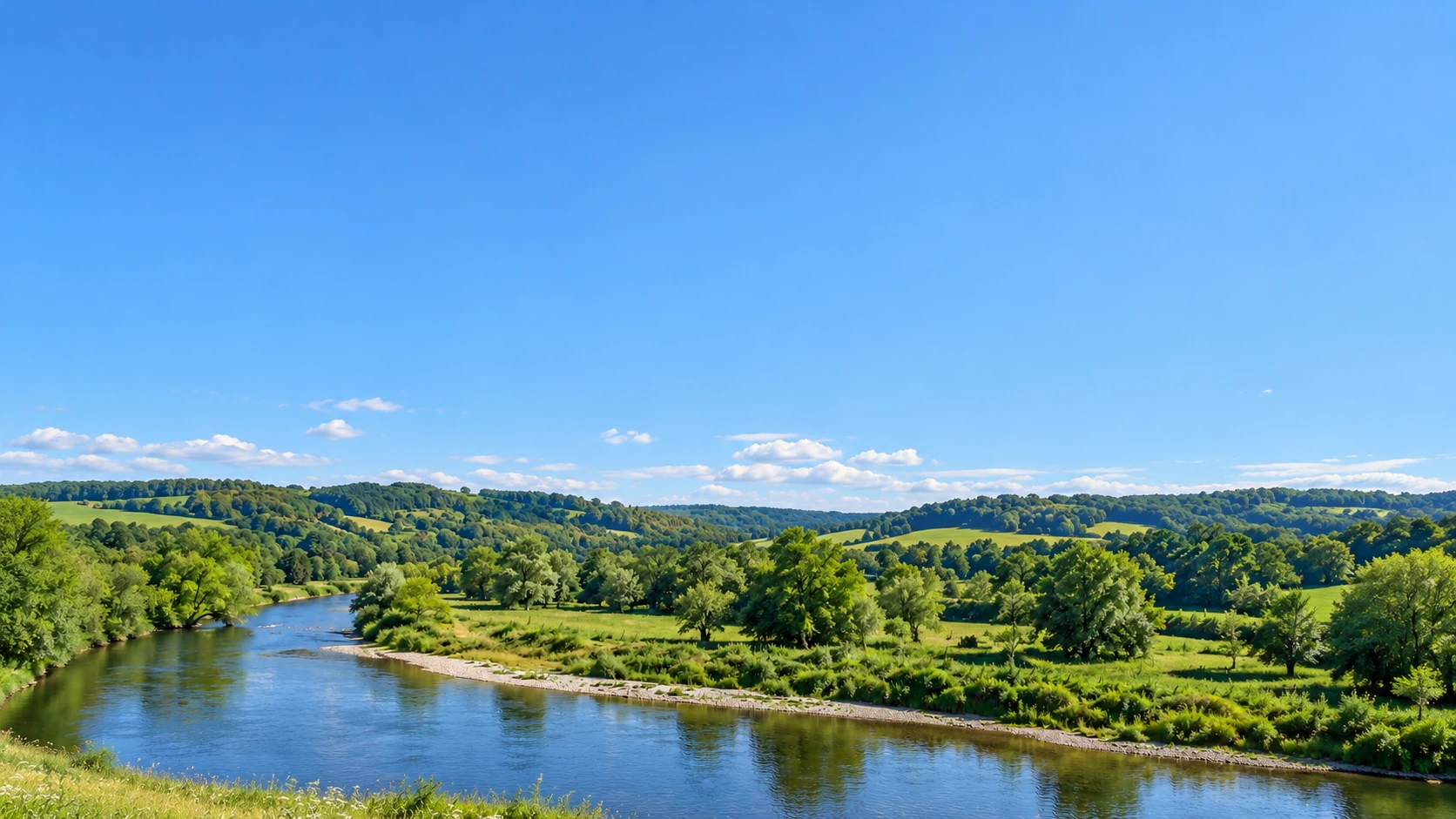
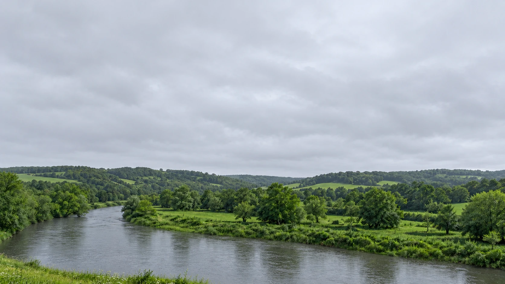
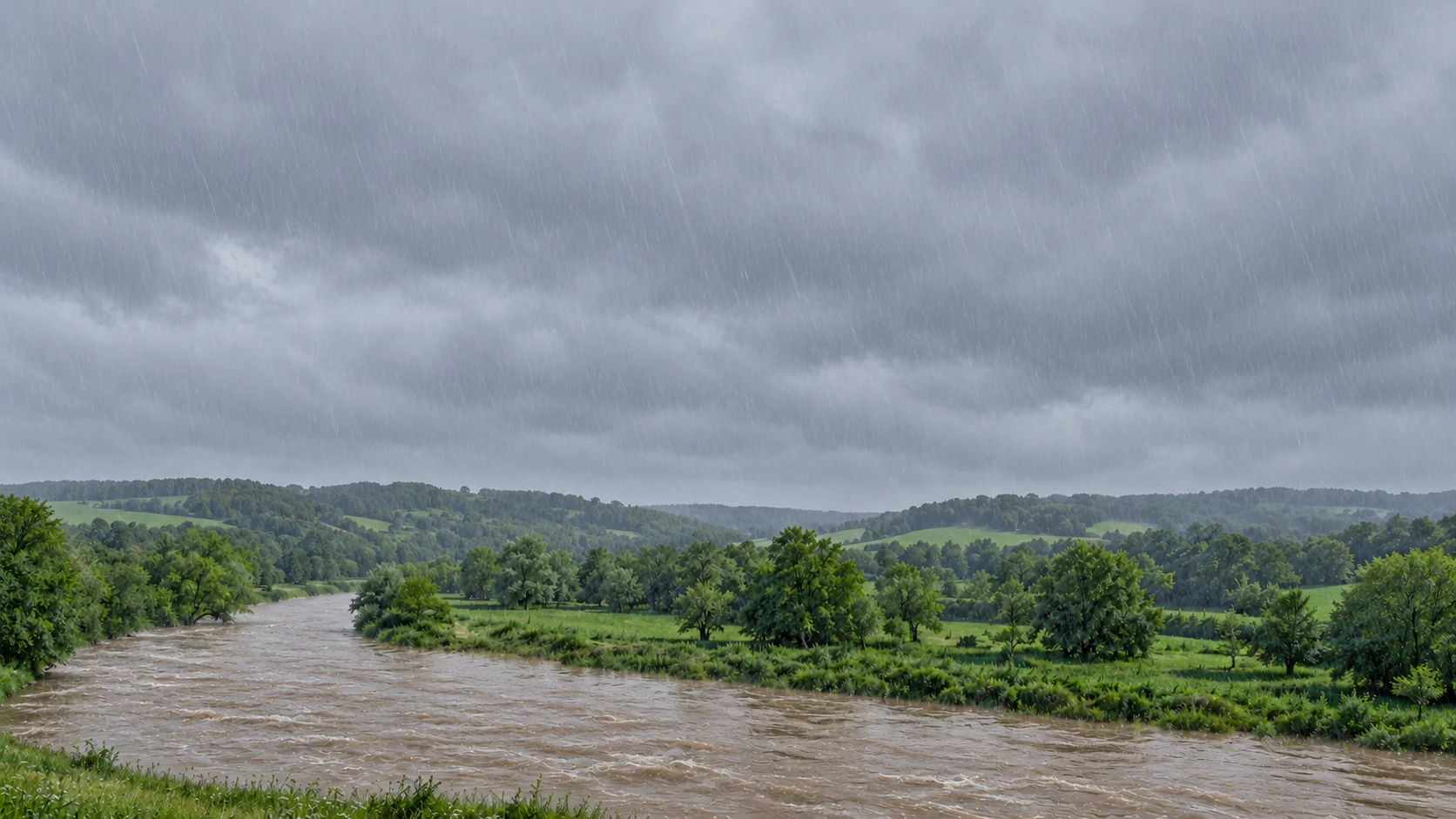
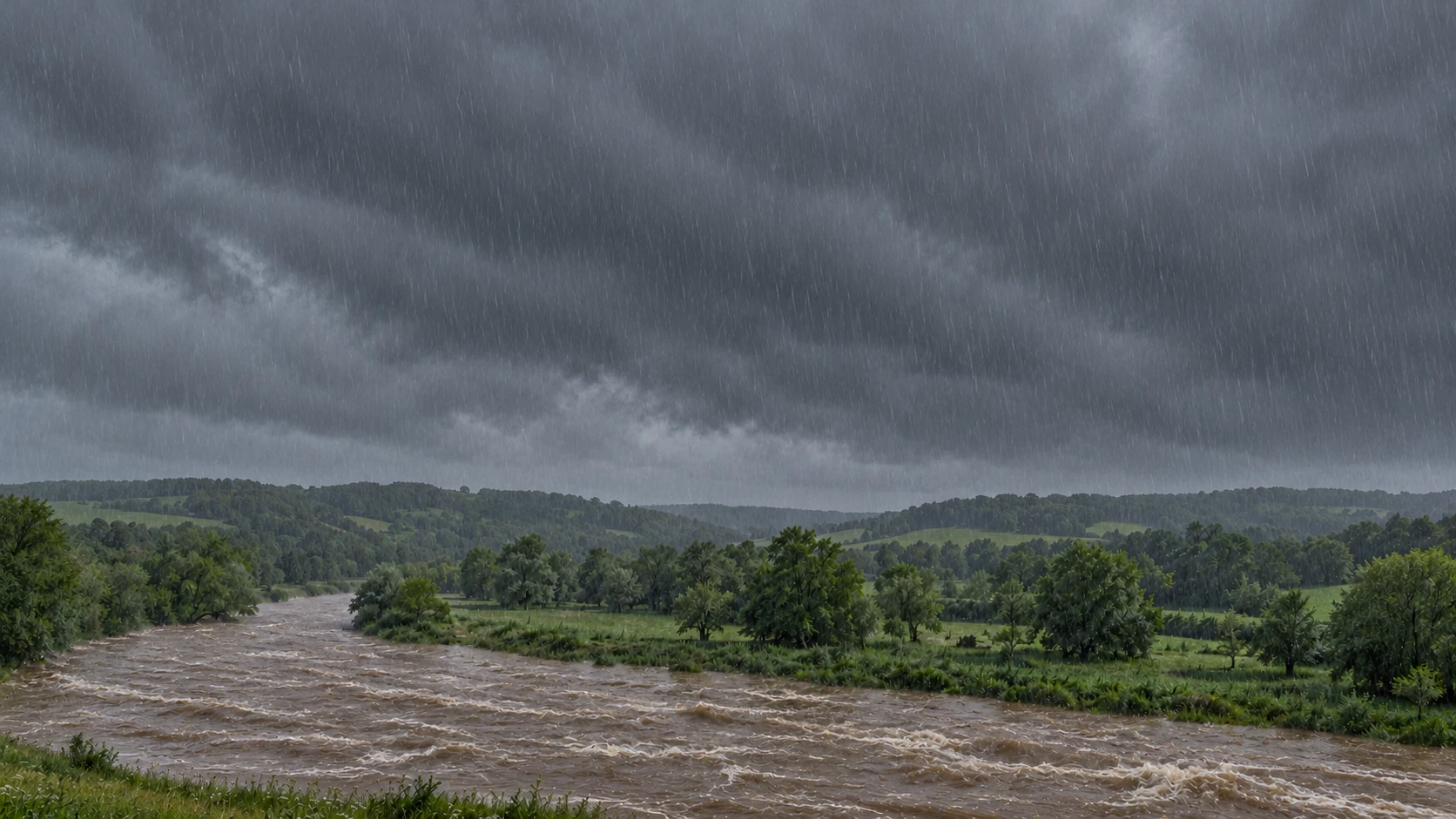
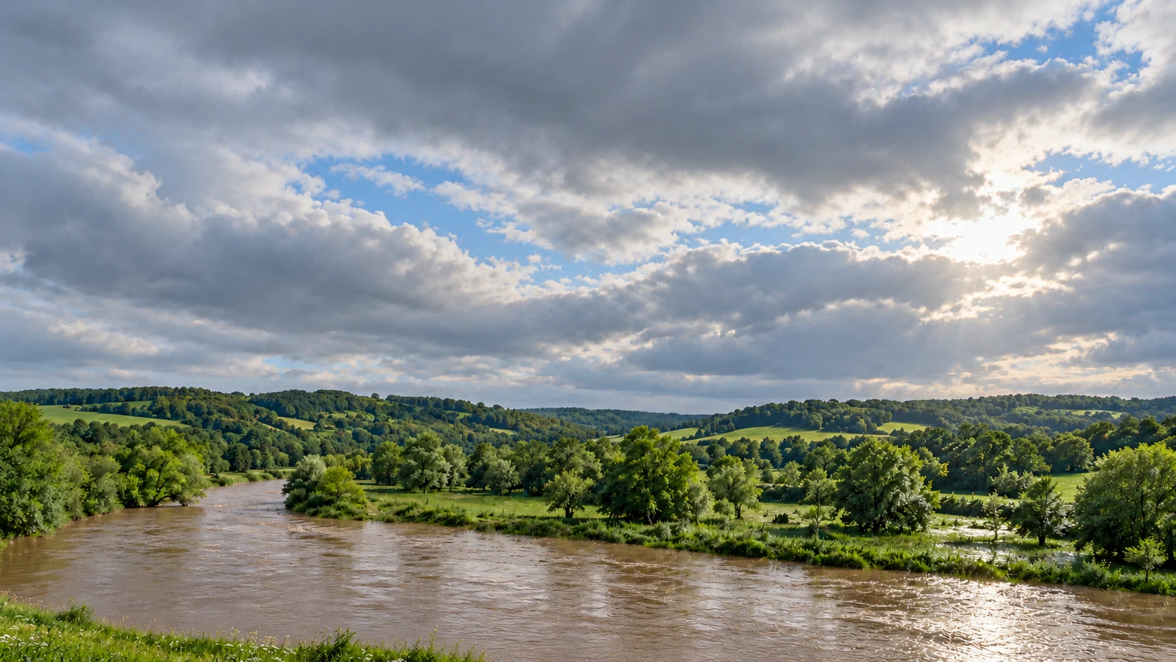
Drag the round handle to explore. Or use the arrow keys to move between weather stages.
Illustrative sequence, not live readings or a weather forecast. Values are fictional; timing varies by catchment. DOC is shown as an optical equivalent (DOCeq).
Clear skies aren’t
the whole picture.
In this example, turbidity falls as the storm eases, while DOC continues to rise. Reading both signals helps explain why the water still needs attention.
The final step represents a later recovery, not an immediate return to normal when the sun appears.
About this example
Based on Roger’s meeting explanation. This interactive example is part of the PMA Compass website, with fictional values and a fixed-camera weather sequence. Weather is context for the story: it is not used here to calculate a dose or predict a plant reading.
Research documents event-specific differences in the timing of turbidity and organic signals. It does not imply that every river behaves this way.
Research: storm-event optical measurements ↗Lutra: Wainuiomata example ↗